Sometime in the next fifteen years, a house will build itself. An AI will draw the design, the structure, the services, and the permit set in an afternoon. The components will come out of an automated factory that runs lights-out. Self-driving trucks will carry the modules to the lot, a robotic crane will set them, and a crew of machines will finish the connections. No clipboard, no subcontractor no-show, no weather delay. The thing assembles itself.
When a good becomes that much cheaper to make, its price falls — the way the price of computation fell, and light, and food before it. The interesting question is not whether this will happen. It is where the money goes when it does. If anyone can build a good house cheaply, who gets rich?
The intuitive answer is that the value flows to two places: to the consumer, as cheaper and better housing, and to the orchestrator who integrates design, factory, logistics, and assembly into one machine, while the component makers earn an ordinary profit. That is broadly right, but it is a description, not an explanation. Cost collapses have swept through industry after industry, and each time the same argument about value and jobs gets had again from scratch. There is a fundamental process at work, and it is old. This essay names it, quantifies it for housing, and follows it to a conclusion sharper than the intuitive answer.
The short version: automation does not destroy value; it moves it. It competes away the margin on everything it touches and pushes the surplus toward whatever stays scarce. In housing, the thing that stays scarce is not the house. It is a particular kind of land — and the permission to build on it. And the process has a shape. It is a smile.
1. The fundamental process: profit runs to whatever stays scarce
Start with a piece of strategy folklore that turns out to be deep. In 2002 the programmer Joel Spolsky wrote down a rule that smart companies follow: "Smart companies try to commoditize their products' complements."[1] A complement is something you buy alongside another thing — cars and gasoline, phones and apps. His mechanism is plain microeconomics: "Demand for a product increases when the prices of its complements decrease." Drive the price of the complement toward zero and the demand — and the pricing power — concentrates on whatever you still control.
Clayton Christensen made the same observation a law of value chains. In The Innovator's Solution he argued that when one stage of a chain becomes modular and commoditized — when its profits are competed away — "the opportunity to earn attractive profits with proprietary products will usually emerge at an adjacent stage."[2] Profit is conserved, but it does not stay put. It migrates to the part of the chain that is still hard, still scarce, still integrated.
The shape this traces is what Stan Shih, the founder of Acer, christened the "smiling curve" around 1992. Plot value-added against the stages of production and you get a smile: the high-value ends are the intangibles — design and R&D at the front, brand and service at the back — while the middle, the actual manufacturing and assembly, sits in the trough.[3] As assembly commoditizes, value slides down the curve toward the ends and outward toward the customer. Automating construction is, precisely, an assault on the middle of the smile.
Now the empirical punchline, and it is startling. The economist William Nordhaus went looking for who actually captures the gains from innovation. Studying U.S. non-farm businesses from 1948 to 2001, he concluded that "only a miniscule fraction of the social returns from technological advances over the 1948–2001 period was captured by producers."[4] His central estimate: innovators keep about 2.2% of the total social value they create. The other ~98% flows to consumers, as lower prices and better products.
Put these together and the process is clear. When you automate a stage of production, you do not get to keep the savings. Competition drags the price of that stage down toward its new, lower cost, and hands the surplus to the customer. The only way to keep economic profit is to own something that cannot be automated or reproduced — the scarce thing at the end of the smile. So the real question is not "who makes the money?" It is: after we automate the building of houses, what is still scarce?
2. It has happened before
Before modelling housing, it is worth establishing that this is a pattern, not a guess. Four episodes, all with hard numbers.
| Episode | What automation did to cost | What happened to volume / value |
|---|---|---|
| Ford Model T (1908–1927) | Moving assembly line (from Oct 1913) cut the price from ~$825–$850 at launch to $260 by 1925[5] | Over 15 million produced; the car went from luxury to mass good — value to consumers |
| U.S. agriculture (1900–2000) | Mechanization collapsed labor per unit of output | Farm share of the workforce fell from 41% (1900) to 1.9% (2000) while output "grew dramatically"[6] |
| Artificial light (industrial age) | Successive lighting technologies | The true price of light fell so far that conventional price indexes understate the gain by a factor of 900–1,600[7] |
| ATMs & bank tellers (1988–2004) | ATMs cut the tellers needed per branch from 20 to 13 | Cheaper branches → banks opened 43% more of them → total teller jobs did not fall[8] |
Every row tells the same story. Cost collapses. Volume explodes. The consumer captures most of the surplus — Nordhaus's 2.2% in microcosm. The share of labor, or of any single input, falls; but because the market expands, the absolute quantity of activity, and often of jobs, holds or grows. And the durable profits accrue not to the thing that got automated but to whatever remained scarce around it: prime farmland, brands, distribution, real estate.
Nordhaus's lighting result deserves a moment, because it is the smile at its most extreme. He found the labour price of light fell from about 58 hours of work per 1,000 lumen-hours for an open fire, and 41 hours for a Babylonian oil lamp around 1750 B.C., to 0.000119 hours for a 1992 compact fluorescent[7:1] — a fall of several hundred thousand-fold. Almost none of it accrued to lamp-makers. It became consumer surplus so vast our statistics can barely see it. That is the prize automation hands the public, and it is the reason to want it.
3. A quantitative anatomy of a house
To see where the surplus goes in housing, start with where the money goes today. The NAHB's Cost of Constructing a Home in 2024 survey gives the anatomy of the average new U.S. single-family home, which sold for $665,298:[9]
| Component | Share of price | Dollars |
|---|---|---|
| Construction (hard cost) | 64.4% | $428,215 |
| Finished lot (land) | 13.7% | $91,057 |
| Overhead & general | 5.7% | $37,922 |
| Sales commissions | 2.8% | $18,628 |
| Financing | 1.5% | $9,979 |
| Marketing | 0.8% | $5,322 |
| Builder profit (pre-tax) | 11.0% | $72,971 |
The first thing to notice is that construction is the whole game: 64.4% of the price — a record high in the survey's history — is the hard cost of actually building. Globally, construction labor productivity has grown about 1% a year over two decades, against 2.8% for the whole economy and 3.6% for manufacturing; closing that gap is a roughly $1.6 trillion opportunity.[10] That 64.4% block is exactly what the automated stack attacks.
Now apply the stack. I model it as a transparent, deliberately illustrative scenario — not a forecast — with every assumption on the table:
| Cost block | Reduction | Rationale |
|---|---|---|
| On-site / assembly labor | −65% | Robotics + factory pre-assembly removes most site labor |
| Materials & components | −20% | Factory precision, waste reduction, standardized parts, bulk buying |
| Equipment | −10% | Modest |
| Overhead & design | −35% | AI design approaches free; platform overhead |
| Sales commissions | −50% | Direct / platform sales |
| Financing | −55% | Build time collapses, so carrying cost collapses |
| Marketing | −35% | Platform distribution |
| Finished lot (held fixed here) | −0% | Treated as fixed for now — a conservative choice revisited in §4 |
The arithmetic is the argument. Hard cost falls from $428k to about $268k. Soft costs fall ~42%. Hold the lot fixed, let the orchestrator earn a normal 8% margin, and the price of the average home falls from $665,298 to about $436,000 — a 34.5% cut.
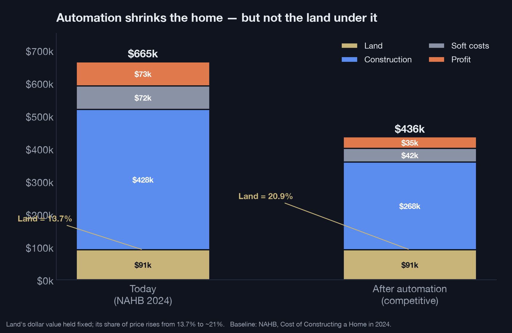
Look at what happened to land. Its dollar value did not change — but because everything else shrank, its share of the price rose from 13.7% to about 21%. That is the fundamental process made visible: automation is a machine for turning the cost of a house into consumer surplus, and the residue it leaves behind is land.
Where did the original $665,298 go? Splitting today's price across the players in the automated, competitive world:
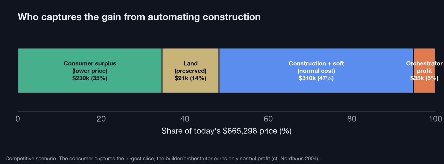
The consumer captures the largest single slice — roughly $230,000 per home, about 35% of today's price. The builder-orchestrator, in competition, earns less in absolute dollars than the builder does today (~$35k vs ~$73k), because competition does to their margin exactly what it does to everyone else's. This is Nordhaus's 2.2% staring back: the people who automate construction will, in the long run, keep very little of the value they unlock. Almost all of it goes to the household — and to the owner of whatever is still scarce.
4. Two kinds of land
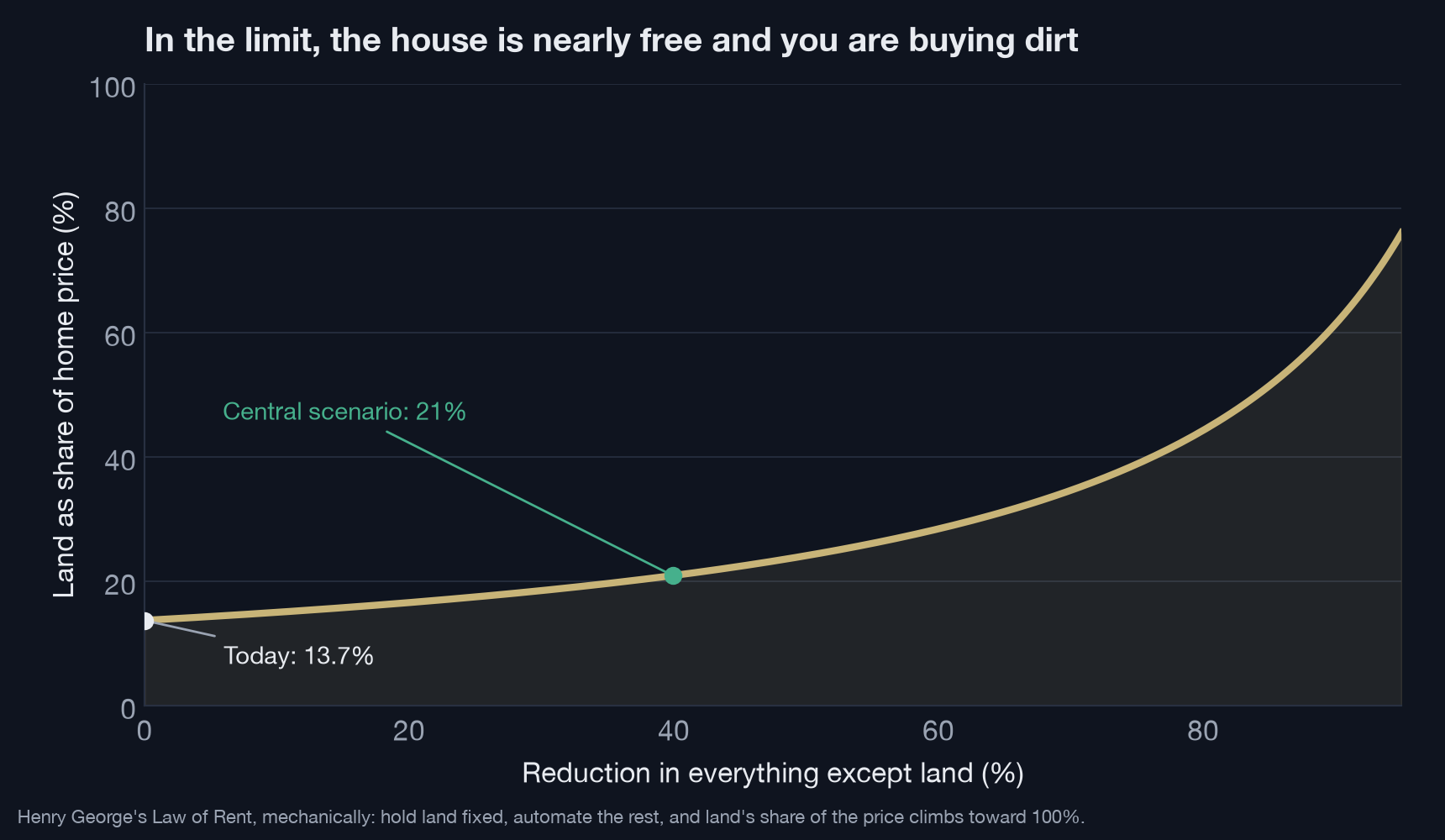
The obvious candidate for "still scarce" is land, and the naïve reading of §3 is that landowners inherit the earth. In 1879 Henry George built an entire political economy on that intuition. His "Law of Rent" held that "wages and interest do not depend on what labor and capital produce — they depend on what is left after rent is taken out."[11] Land, fixed in supply, is the residual claimant; whatever surplus a more productive economy throws off, the owner of the scarce site captures by charging more for access. Run the model of §3 to its limit and George's logic becomes mechanical: hold land fixed, keep automating everything else, and land's share of the home price climbs toward 100%.
But "land" is not one thing, and this is where the intuitive story goes wrong. The NAHB's "finished lot" is not raw ground. It is raw ground plus the horizontal construction that turns it into a buildable lot: clearing, grading, trenching, roads, water, sewer, power, drainage. Development is itself construction — and construction is exactly what automation makes cheap. Autonomous graders, trenching robots, automated road-laying and utility installation attack the finished lot from the inside. A "finished lot," in other words, splits into two very different things:
- a reproducible part — the site development, which automation collapses like any other construction; and
- a non-reproducible part — the raw location value and the legal permission to build, which no robot can manufacture.
Once you make that split, the picture changes depending on where you are building.
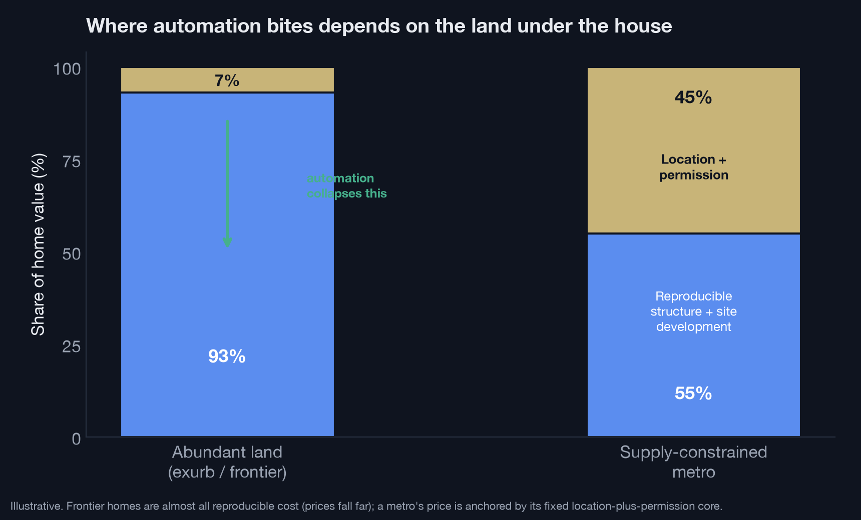
At the frontier — the exurban and greenfield land that is cheap precisely because it is abundant — a home is almost entirely reproducible cost. Raw land is a rounding error; most of what makes a lot expensive is the development. Automate the development and frontier lots get dramatically cheaper. This is not a small effect. Cheaper site work, combined with cheaper logistics and eventually autonomous transport, pushes the margin of settlement outward — the classic bid-rent logic that runs from von Thünen to Alonso.[12] Land that was uneconomic to develop becomes economic. The effective supply of buildable land expands. Far from enriching frontier landowners, automation deflates frontier land, because their land was expensive only in proportion to the cost of taming it, and that cost is now falling.
In the supply-constrained metro, the story is the opposite. There, a large share of a home's value is not development cost at all; it is location — proximity, amenity, access to jobs — and the regulatory right to build, which zoning and entitlement deliberately keep scarce. Automation cannot touch either. So the George trap is real, but it is local: it binds only where the non-reproducible core is large and supply is legally frozen. And even there, it is fought by the frontier effect — cheaper development elsewhere expands the menu of places people can live, which competes against the scarce metro location.
The refined conclusion, then, is not "landowners win." It is narrower and more useful: the durable rent accrues to location plus permission, in the specific places where permission is withheld. Automation makes structures cheap, makes developable land cheaper, and pushes the frontier out. The one thing it cannot make is the legal right to build where people most want to live. That is why the fight will move, over the next two decades, from the cost of building to the cost of the right to build.
5. Who claims the Schumpeterian rent?
The steady state — cheap homes, surplus to consumers, rent to constrained-metro location — is fifteen or twenty years out. Between here and there lies a generation of transition, and transitions are where fortunes are actually made. Joseph Schumpeter named the prize: the innovator earns a temporary, above-normal profit — a Schumpeterian rent — for being first, and competition then erodes it through imitation, the process he called creative destruction.[13] Nordhaus's 2.2% is what survives to the steady state; the transitional rent, earned before prices fall to the new marginal cost, is enormous in absolute terms even as, per innovation, it melts. Who claims it?
Not one party. It is handed down a line, like a baton. The bottleneck — the thing that is scarce at that moment — moves over the course of the transition, and the rent moves with it.
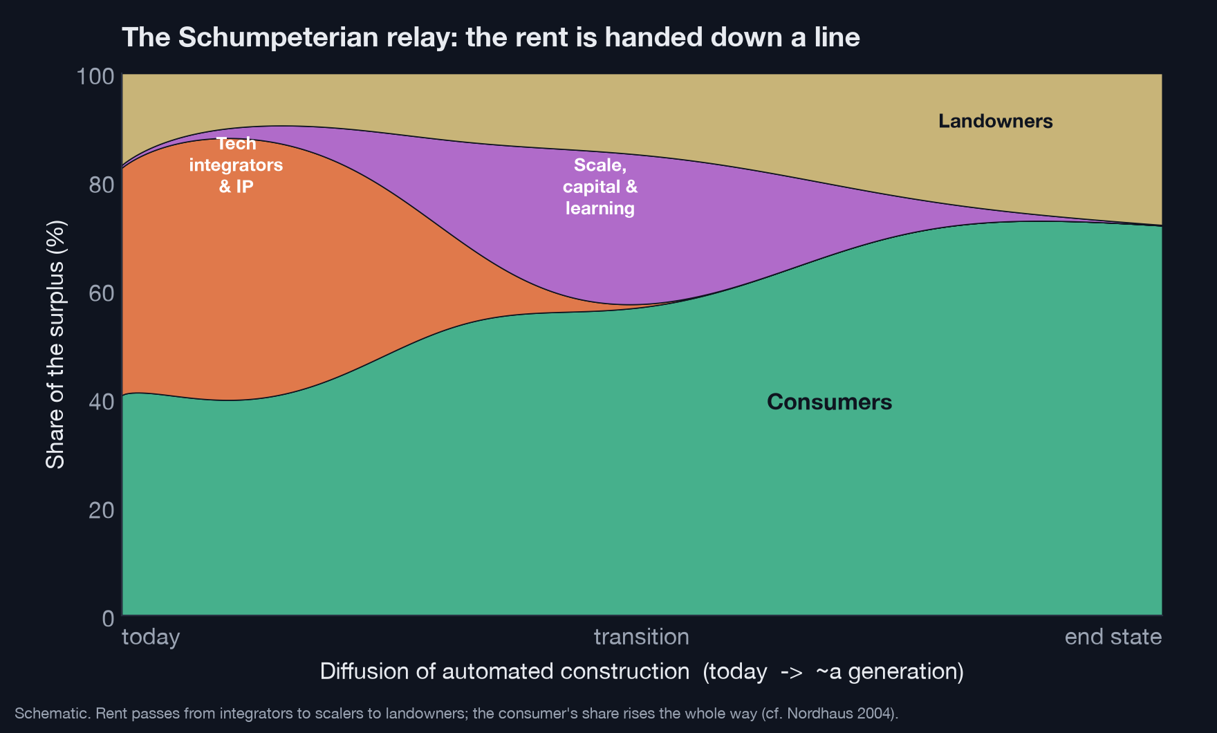
- Early — the technologists. At first the scarce thing is the working stack itself: the design AI, the robotics, the factory integration, the software that ties modular pieces into a delivered house. The first firms to assemble it earn the classic entrepreneur's rent, protected for a while by IP and know-how. But the components — models, robots, logistics — are advancing broadly and are themselves modular, so imitation comes fast and this rent is the first to fade.
- Middle — scale, capital, and the learning curve. As the technology diffuses, advantage shifts from having it to scaling it. Factories and robot fleets are capital-intensive, so patient capital earns a return; and, as James Bessen documents, cumulative production builds a cost advantage through learning by doing[8:1] that the first mover to scale can hold. Two scarce assets become decisive here: entitled-land pipelines and regulatory approvals (building-code and factory-built-housing certification). This is why incumbents with balance sheets and land banks — large builders, private equity, infrastructure capital — are well positioned to capture the middle of the relay, precisely by combining cheap automated building with land and permits they already hold.
- Late — the landowners. Once the technology and the scaling both commoditize, the only scarcity left is the one from §4: location plus permission. The rent settles there. This is the George steady state, and it is where the durable, un-competed-away return finally comes to rest.
Underneath all of it, the consumer's share rises the whole way — the relay is a story about who skims the transitional surplus, but the surplus itself is flowing, monotonically, to households, exactly as Nordhaus predicts. Some transitional rent also accrues to scarce skilled labor — the robot technicians, integration engineers, and factory operators who are in short supply early and command a wage premium (David Autor's complementarity, of which more below[14]) — but that too erodes as training catches up.
The strategic lesson is uncomfortable and clarifying. The transitional rent is a melting ice cube. The way to make it durable is to convert it, while you hold it, into a position in the one thing that does not melt: location and permission. The smart money grabs the integration rent early and parlays it into entitled land and distribution before competition takes the rent away. Whether the integration layer itself can hold rent longer depends on market structure — genuine network effects or scale economies could let a few platforms behave like Christensen's integrated layer and keep a margin; a modular, competitive stack dissipates the rent to consumers quickly. Either way, the terminal owner of the surplus is not the roboticist. It is the household, and the landowner in the places we refuse to let grow.
6. The jobs question, answered with arithmetic
The loudest fear about construction automation is jobs. It is also the most answerable, because it is just multiplication. Sector employment equals labor per home × homes built. Automation cuts the first term. Whether total employment falls depends entirely on the second.
Suppose automation cuts labor per home by 55% (a central guess; the chart also shows −40% and −65%). To hold construction employment flat, the number of homes built must rise by 1 ÷ (1 − 0.55) = 2.22×, i.e. +122%. Does demand rise that much?
From price alone, no. With a 34.5% price cut and a long-run price elasticity of housing demand around −0.7 — squarely within the −0.5 to −0.8 range the empirical literature has clustered on for decades[15] — quantity demanded rises only about +24%, well short of the +122% needed.
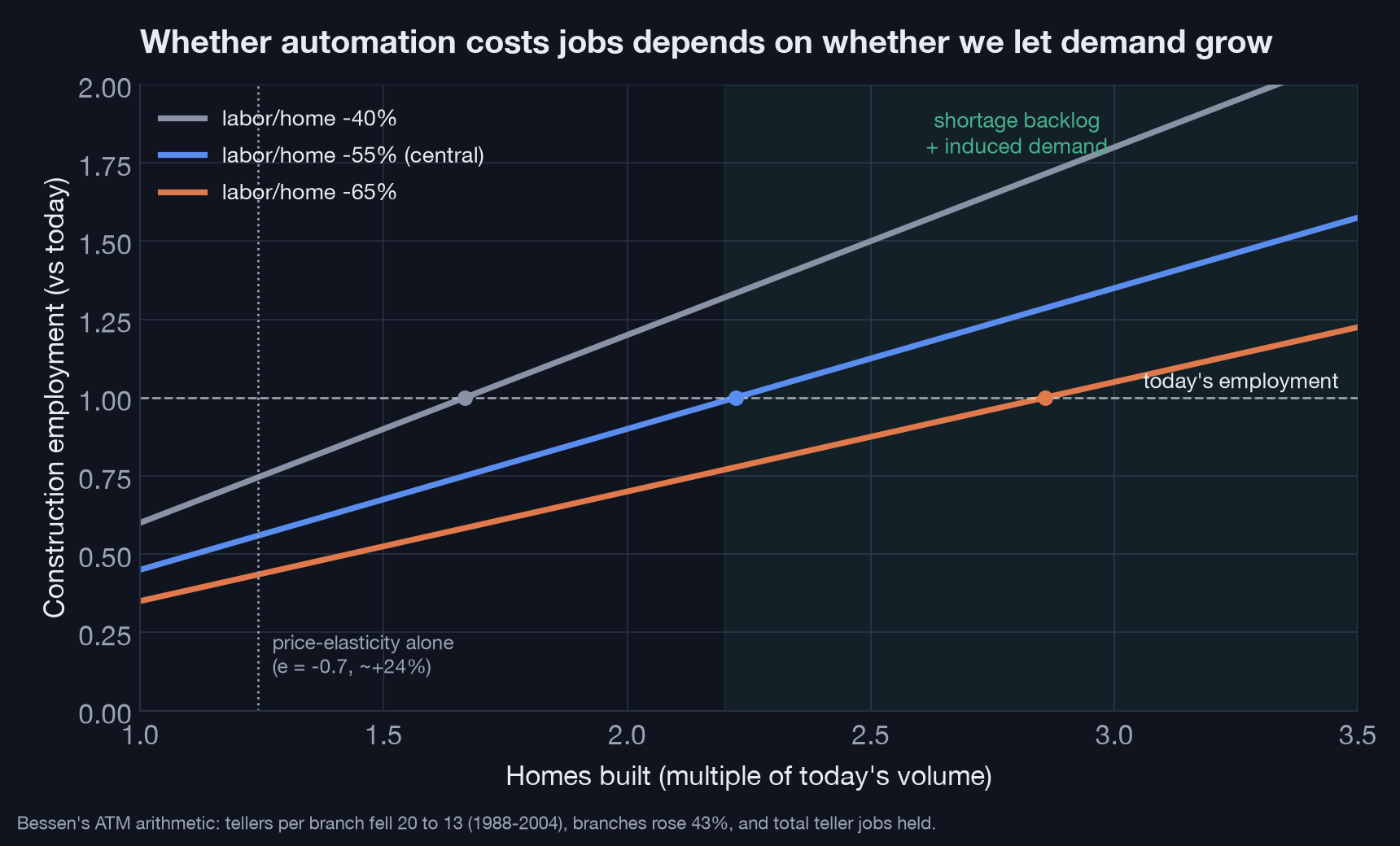
But price elasticity is the smallest part of the demand response, for three reasons.
First, there is a backlog. The U.S. is estimated to be short roughly 3.5–3.9 million homes — Freddie Mac put the deficit at 3.8 million units as of 2020, and Up for Growth measured underproduction at 3.85 million.[16] That is enormous pent-up demand waiting for prices to fall.
Second, there is induced demand — the Jevons effect. In 1865, studying coal, William Stanley Jevons demolished the intuition that efficiency reduces consumption: "It is wholly a confusion of ideas to suppose that the economical use of fuel is equivalent to a diminished consumption. The very contrary is the truth."[17] When something gets dramatically cheaper, we find far more uses for it. Cheap construction does not just sell the same houses for less; it unlocks teardown-and-rebuilds, accessory dwelling units, second homes, bigger homes, earlier household formation, and building in places that were previously uneconomic — the very frontier expansion of §4. The elasticity measured on today's expensive, constrained market badly understates the response to an order-of-magnitude change.
Third, this is the Bessen ATM pattern exactly. When ATMs cut the tellers needed per branch from 20 to 13, the naïve forecast was mass teller unemployment. Instead, cheaper branches let banks open 43% more of them, and total teller employment held.[8:2] David Autor's survey of automation reaches the same conclusion: "automation also complements labor, raises output in ways that lead to higher demand for labor… Journalists and even expert commentators tend to overstate the extent of machine substitution for human labor and ignore the strong complementarities between automation and labor."[14:1] The construction worker of the automated era is less likely to swing a hammer and more likely to run a factory line, maintain robots, manage logistics, or design — new tasks created beside the ones automated away.
So the honest answer on jobs is conditional, and the condition is the one from §4: employment holds if and only if we let volume expand — which requires land to build on and permission to build. Automate construction but freeze the supply of buildable land, and you get the worst of both worlds: displaced labor and inflated location rents, with the consumer surplus captured on the way. Let building rip, and you get cheaper homes, sustained employment, and the surplus reaching households. The technology does not decide which world we get. Zoning does.
7. So, who makes the money?
Here is the fully assembled answer.
- The consumer wins biggest, and permanently. Most of the surplus from automating construction flows to households as cheaper, better housing — on the order of $200k+ per home in the model, consistent with Nordhaus's finding that innovators keep barely 2% of what they create. This is the most reliable prediction in the essay, and it is the point of the whole exercise.
- The transitional rent is a relay, and it is worth chasing. Over the next generation, real fortunes will be made — first by the technologists who assemble the stack, then by whoever scales it with capital, learning, and entitled land. But each holder's rent melts as the next bottleneck takes over. To keep it, convert it into the one asset that stays scarce.
- The durable rent is location plus permission — but only where we withhold permission. Automation makes structures cheap, makes developable land cheaper, and pushes the frontier out. It cannot make the legal right to build where people most want to live. That is the true residual claimant, and it is a policy choice, not a law of nature.
- Jobs need not fall. Component makers earn ordinary profit; construction employment holds if demand expands enough — the Bessen arithmetic — while the work shifts from the trough of the smile (site labor) toward its ends (factories, robotics, logistics, design).
The intuitive answer — consumer and orchestrator — was right about the consumer and half-right about the orchestrator, whose prize turns out to be real but temporary. What it missed is the deepest player: land, and the rules that govern it. The fundamental process — value running to whatever stays scarce — predicts that automation will make the house the cheap part and move the whole contest to the ground beneath it and the permission slip to put something there.
Which returns us to the title. Robots will push value down the smiling curve, away from the commoditized middle and out to the ends — and past the ends, to the household. The surplus they create is a smile in the most literal sense: the same kind of gain that took light from 58 hours of labor to a fraction of a second, arriving now for shelter. We will get it — cheaper, better, more abundant housing — if we let the machine build, and let it build where people actually want to live. Build the machine that builds the houses. Then, just as urgently, free the land for it to build on.
A note on method
The cost anatomy in §3 uses the NAHB's 2024 builder survey for the baseline.[9:1] The automation scenario, the split of the finished lot into reproducible development and a non-reproducible location-plus-permission core (§4), and the two-regime and relay figures (§4–§5) are explicit, labeled illustrative constructions — laid out so the reader can disagree with any number. The qualitative results — a large consumer surplus, a falling price, a rising share for the non-reproducible core, frontier land getting cheaper, a transitional rent that melts, and jobs that hinge on volume — follow from the structure (some things are reproducible and collapse; location and permission are not and do not), not from the exact percentages. The employment model is the simplest possible identity, jobs = labor-per-home × homes-built, to keep the break-even logic transparent. None of this forecasts a particular year; it is an argument about direction.
References
Joel Spolsky, "Strategy Letter V," Joel on Software, June 12, 2002. https://www.joelonsoftware.com/2002/06/12/strategy-letter-v/ ↩︎
Clayton M. Christensen and Michael E. Raynor, The Innovator's Solution (Harvard Business School Press, 2003) — the "law of conservation of attractive profits": when modularity and commoditization erase profit at one stage, the chance to earn attractive profits emerges at an adjacent stage. Discussed in Ben Thompson, "Netflix and the Conservation of Attractive Profits," Stratechery, 2015. https://stratechery.com/2015/netflix-and-the-conservation-of-attractive-profits/ ↩︎
The "smiling curve" was proposed c. 1992 by Stan Shih, founder of Acer. See Ming Ye, Bo Meng, and Shang-Jin Wei, "Measuring Smile Curves in Global Value Chains," Oxford Bulletin of Economics and Statistics 82(5): 988–1016 (2020), doi:10.1111/obes.12364; and https://en.wikipedia.org/wiki/Smiling_curve ↩︎
William D. Nordhaus, "Schumpeterian Profits in the American Economy: Theory and Measurement," NBER Working Paper No. 10433 (2004): "only a miniscule fraction of the social returns from technological advances over the 1948–2001 period was captured by producers." Central estimate ≈ 2.2% (U.S. non-farm business). https://www.nber.org/papers/w10433 ↩︎
"Ford Model T," Wikipedia (accessed 2026), corroborated by HISTORY.com: launch price ~$825 (1909 Runabout) to ~$850 (1908); lowered to $260 by 1925; over 15 million produced from October 1, 1908 to May 26, 1927; the moving assembly line began October 7, 1913. https://en.wikipedia.org/wiki/Ford_Model_T ↩︎
Carolyn Dimitri, Anne Effland, and Neilson Conklin, "The 20th Century Transformation of U.S. Agriculture and Farm Policy," USDA Economic Research Service, Economic Information Bulletin No. 3 (2005): agriculture employed 41% of the workforce in 1900, falling to 16% (1945), 4% (1970), and 1.9% (2000), while "output from U.S. farms has grown dramatically." https://www.ers.usda.gov/publications/pub-details/?pubid=44198 ↩︎
William D. Nordhaus, "Do Real-Output and Real-Wage Measures Capture Reality? The History of Lighting Suggests Not," in T. Bresnahan and R. Gordon (eds.), The Economics of New Goods (University of Chicago Press / NBER, 1996), pp. 27–70: traditional price indexes overstate the true price of light — equivalently understate the growth in lighting — by a factor of 900 to 1,600 since the start of the industrial age; in labor terms the price of light fell from ~58 hours of work per 1,000 lumen-hours (open fire) and ~41 hours (Babylonian lamp, 1750 B.C.) to 0.000119 hours for a 1992 compact fluorescent. https://www.nber.org/system/files/chapters/c6064/c6064.pdf ↩︎ ↩︎
James Bessen, "Toil and Technology," Finance & Development (IMF), Vol. 52, No. 1 (March 2015): the number of tellers per urban branch fell from 20 to 13 between 1988 and 2004, but urban bank branches rose 43% (with over 400,000 ATMs installed), so total teller jobs did not disappear. See also Bessen, Learning by Doing: The Real Connection between Innovation, Wages, and Wealth (Yale University Press, 2015) on learning-curve cost advantages. https://www.imf.org/external/pubs/ft/fandd/2015/03/bessen.htm ↩︎ ↩︎ ↩︎
Eric Lynch, "Cost of Constructing a Home in 2024," NAHB (January 20, 2025): average new single-family sale price $665,298; construction costs 64.4%, finished lot 13.7%, overhead 5.7%, sales commissions 2.8%, financing 1.5%, marketing 0.8%, builder profit 11.0% (pre-tax); long-run average pre-tax profit share since 1998 is 9.8%. Self-reported builder survey. https://eyeonhousing.org/2025/01/cost-of-constructing-a-home-in-2024/ ↩︎ ↩︎
McKinsey Global Institute, Reinventing Construction: A Route to Higher Productivity (February 2017): "construction sector labor-productivity growth averaged 1 percent a year over the past two decades, compared with 2.8 percent for the total world economy and 3.6 percent for manufacturing"; ~$10 trillion is spent on construction-related goods and services each year; closing the gap could add ~$1.6 trillion. (Figures are global and reflect a ~1997–2017 average.) https://www.mckinsey.com/capabilities/operations/our-insights/reinventing-construction-through-a-productivity-revolution ↩︎
Henry George, Progress and Poverty (1879), Book III, "The Law of Rent": "wages and interest do not depend on what labor and capital produce — they depend on what is left after rent is taken out." George's empirical claim that rent necessarily absorbs productivity gains was contested by later economists (Marshall, Young, Ely); it is used here as a framework, not settled law. https://www.henrygeorge.org/pchp11.htm ↩︎
The frontier argument follows the bid-rent tradition of Johann Heinrich von Thünen, The Isolated State (1826), and William Alonso, Location and Land Use (Harvard University Press, 1964): cheaper development, transport, and access push the margin of profitable settlement outward and lower land rents at the frontier. ↩︎
Joseph A. Schumpeter, Capitalism, Socialism and Democracy (Harper & Brothers, 1942) — the theory of "creative destruction": entrepreneurial innovation earns a temporary, above-normal profit that competition and imitation subsequently erode. The Schumpeterian rent measured empirically in the steady state is Nordhaus's ~2.2% (see above). ↩︎
David H. Autor, "Why Are There Still So Many Jobs? The History and Future of Workplace Automation," Journal of Economic Perspectives 29(3): 3–30 (Summer 2015), doi:10.1257/jep.29.3.3: "automation also complements labor, raises output in ways that lead to higher demand for labor… Journalists and even expert commentators tend to overstate the extent of machine substitution for human labor and ignore the strong complementarities between automation and labor that increase productivity, raise earnings, and augment demand for labor." https://www.aeaweb.org/articles?id=10.1257/jep.29.3.3 ↩︎ ↩︎
Stephen K. Mayo, "Theory and Estimation in the Economics of Housing Demand," Journal of Urban Economics 10(1): 95–116 (1981), reviewing the literature: price elasticity of housing demand estimates cluster around −0.5 to −0.8 (Muth −0.76; Polinsky & Ellwood −0.67/−0.70; Rosen −0.67; Straszheim −0.53) and are almost all inelastic. A point estimate of −0.7 with a sensitivity band of roughly −0.3 to −1.0 is defensible. ↩︎
Sam Khater et al., "Housing Supply: A Growing Deficit," Freddie Mac Economic & Housing Research Note (May 7, 2021): a housing supply deficit of 3.8 million units as of Q4 2020, up ~52% from 2.5 million in 2018. Up for Growth, Housing Underproduction in the U.S., measured underproduction at 3.85 million homes (2022). The two use different methods but cluster in the high-3-million range. https://www.freddiemac.com/research/insight/20210507-housing-supply ↩︎
William Stanley Jevons, The Coal Question (London: Macmillan, 1865; 2nd ed. 1866), Chapter VII, "Of the Economy of Fuel": "It is wholly a confusion of ideas to suppose that the economical use of fuel is equivalent to a diminished consumption. The very contrary is the truth." https://www.econlib.org/library/YPDBooks/Jevons/jvnCQ7.html ↩︎